Stochastic Multiple Target Sampling Gradient Descent

October 27, 2022

1. Introduction

Sampling from an unnormalized target distribution that we know the density function up to a scaling factor is a pivotal problem with many applications in probabilistic inference [1,2]. For this purpose, Markov chain Monte Carlo (MCMC) has been widely used to draw approximate posterior samples, but unfortunately, is often time-consuming and has difficulty accessing the convergence [3]. Targeting an efficient acceleration of MCMC, some stochastic variational particle-based approaches have been proposed, notably Stochastic Langevin Gradient Descent [4] and Stein Variational Gradient Descent (SVGD) [3]. Outstanding among them is SVGD, with a solid theoretical guarantee of the convergence of the set of particles to the target distribution by maintaining a flow of distributions. More specifically, SVGD can be viewed as a probabilistic version of the GD for single-objective optimization.

On the other side, multi-objective optimization (MOO) [5] aims to optimize a set of objective functions and manifests itself in many real-world applications problems, such as in multi-task learning (MTL) [6, 7], natural language processing, and reinforcement learning . Leveraging the above insights, it is natural to ask: “Can we derive a probabilistic version of multi-objective optimization?”. By answering this question, we enable the application of the Bayesian inference framework to the tasks inherently fulfilled by the MOO framework.

In summary, we make the following contributions in this work:

Propose a principled framework that incorporates the power of Stein Variational Gradient Descent into multi-objective optimization. Concretely, our method is motivated by the theoretical analysis of SVGD, and we further derive the formulation that extends the original work and allows to sample from multiple unnormalized distributions.
Demonstrate our algorithm is readily applicable in the context of multi-task learning. The benefits of MT-SGD are twofold: i) the trained network is optimal, which could not be improved in any task without diminishing another, and ii) there is no need for predefined preference vectors as in previous work [6, 8], MT-SGD implicitly learns diverse models universally optimizing for all tasks.
Conduct comprehensive experiments to verify the behaviors of MT-SGD and demonstrate the superiority of MT-SGD to the baselines in a Bayesian setting, with higher ensemble performances and significantly lower calibration errors.

2. Multi-Target Sampling Gradient Descent

2.1 Problem Setting

Given a set of target distributions $p_{1:K}\left(\theta\right):=\{p_{1}(\theta),\ldots,p_{K}(\theta)\}$ , with parameter $\theta$ , we aim to find the optimal distribution $q \in Q$ that minimizes a vector-valued objective function whose k-th component is $D_{KL}(q\Vert p_{k})$ :

$\min_{q\in\mathcal{Q}}\left[D_{KL}\left(q\Vert p_{1}\right),...,D_{KL}\left(q\Vert p_{K}\right)\right]$

where $D_{KL}$ represents Kullback-Leibler divergence and $\mathcal{Q}$ is a family of distributions.

When there exists an objective function that conflicts with each other, there will be a trade-off between these two objectives. Therefore, no “optimal solution” exists in such cases. Alternatively, we are often interested in seeking a set of solutions such that each does not have any better solution (i.e. achieves lower loss values in all objectives) [6-9]. The optimization problem (OP) in (??) thus can be viewed as a multi-objective OP \cite{desideri2012multiple} on the probability distribution space. Let us denote $\mathcal{H}_{k}$ by the Reproducing Kernel Hilbert Space (RKHS) associated with a positive semi-definite (p.s.d.) kernel $k$ , and $\mathcal{H}_{k}^{d}$ by the $d$ -dimensional vector function:

$f=[f_{1},\ldots,f_{d}], (f_{i}\in\mathcal{H}_{k}).$

2.2 Our approach
Inspired by [3], we construct a flow of distributions $q_{0},q_{1},...,q_{L}$ departed from a simple distribution $q_{0}$ , that gradually move closer to all the target distributions. In particular, at each step, assume that $q$ is the current obtained distribution, and the goal is to learn a transformation $T=id+\epsilon\phi$ so that the \emph{feed-forward distribution} $q^{[T]}=T\#q$ moves closer to $p_{1:K}$ simultaneously. Here we use $id$ to denote the identity operator, $\epsilon>0$ is a step size, and $\phi\in\mathcal{H}_{k}^{d}$ is a velocity field. Particularly, the problem of finding the optimal transformation $T$ for the current step is formulated as:

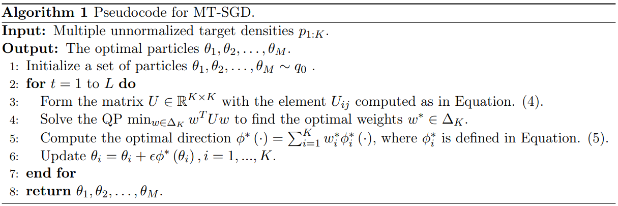
$\min_{\phi}\left[D_{KL}\left(q^{[T]}\Vert p_{1}\right),...,D_{KL}\left(q^{[T]}\Vert p_{K}\right)\right].$

The key steps of our MT-SGD are summarized in Algorithm 1, where the set of particles $\theta_{1:M}$ is updated gradually to approach the multiple distributions $p_{1:K}$ .

Analysis for the case of RBF kernel: We now consider a radial basis-function (RBF) kernel of bandwidth $\sigma$ : $k\left(\theta,\theta'\right)=\exp\left\{-||\theta-\theta'||^{2}/\left(2\sigma^{2}\right)\right\}$ and examine some asymptotic behaviors.

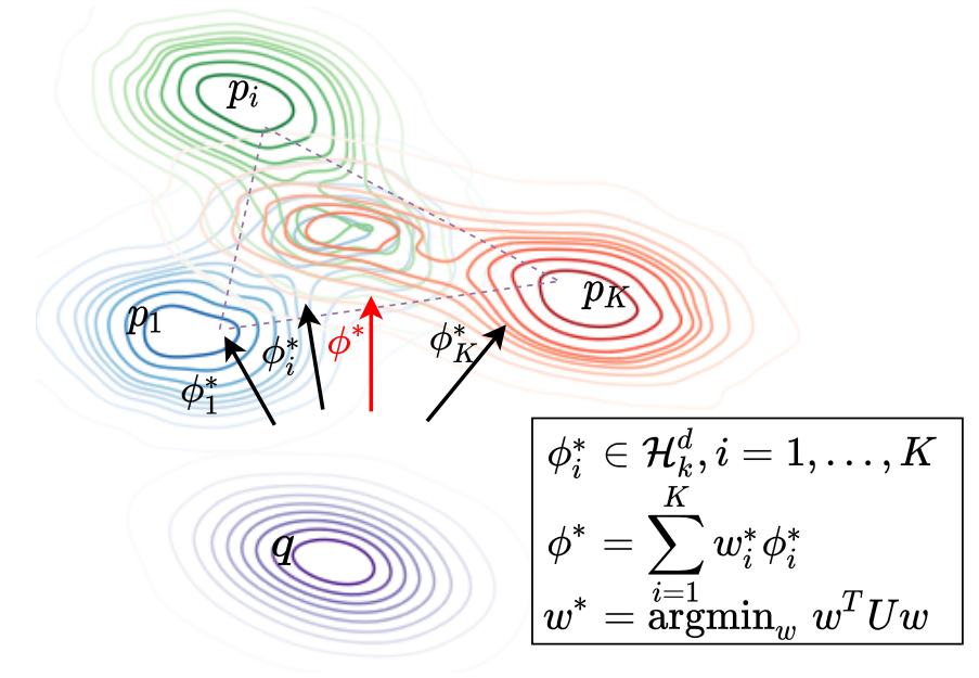
Figure 1: How to find the optimal descent direction

General case: The elements of the matrix $U$ become

$U_{ij} =\mathbb{E}_{\theta,\theta'\sim q}\Biggl[\exp\left\{ \frac{-||\theta-\theta'||^{2}}{2\sigma^{2}}\right\} \Biggl[\left\langle \nabla\log p_{i}(\theta),\nabla\log p_{j}(\theta')\right\rangle$

$+\frac{1}{\sigma^{2}}\left\langle \nabla\log p_{i}(\theta)-\nabla\log p_{j}(\theta'),\theta-\theta'\right\rangle -\frac{d}{\sigma^{2}}-\frac{||\theta-\theta'||^{2}}{\sigma^{4}}\Biggr]\Biggr].$

Single particle distribution $q=\delta_{\theta}$ : The elements of the matrix $U$ become

$U_{ij}=\left\langle \nabla\log p_{i}(\theta),\nabla\log p_{j}(\theta)\right\rangle ,$

When $\sigma\to\infty$ : The elements of the matrix $U$ become

$U_{ij} =\mathbb{E}_{\theta,\theta'\sim q}\Biggl[\left\langle \nabla\log p_{i}(\theta),\nabla\log p_{j}(\theta')\right\rangle \Biggr].$

2.3 Comparison to MOO-SVGD and Other Work

The most closely related work to ours is MOO-SVGD [9]. In a nutshell, ours is principally different from that work and we show a fundamental difference between our MT-SGD and MOO-SVGD in Figure 1. Our MT-SGD navigates the particles from one distribution to another distribution consecutively with a theoretical guarantee of globally getting closely to multiple target distributions. By contrast, while MOO-SVGD also uses the MOO [5] to update the particles, their employed repulsive term encourages the particle diversity without any theoretical-guaranteed principle to control the repulsive term, hence it can force the particles to scatter on the multiple distributions. In fact, they aim to profile the whole Pareto front, which is preferred when users want to obtain a collection of diverse Pareto optimal solutions with different trade-offs among all tasks.

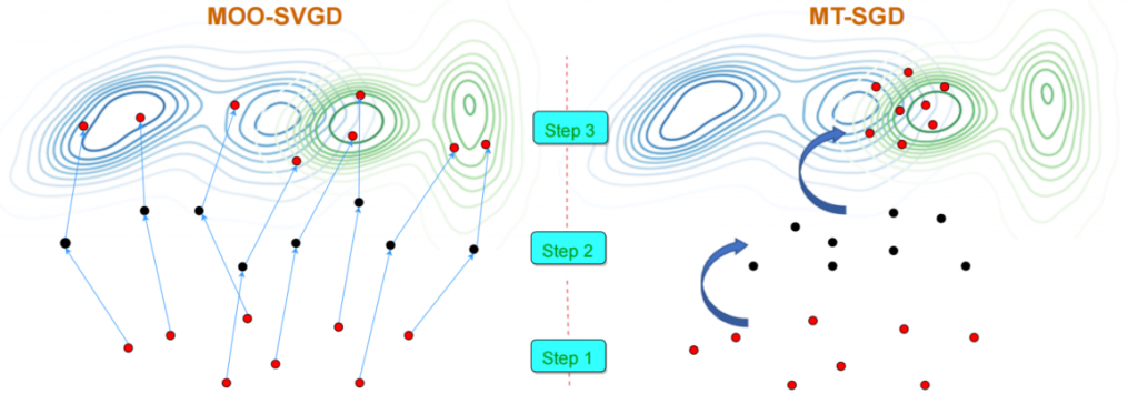
Figure 2: Our MT-SGD moves the particles from one distribution to another distribution to globally get closer to two target distributions (i.e., the blue and green ones). Differently, MOO-SVGD uses MOO to move the particles individually and independently. The diversity is enforced by the repulsive forces among particles. There is no principle to control these repulsive forces, hence they can push the particles scattering on two distributions

3. Experiments

In this section, we verify our MT-SGD by evaluating its performance on both synthetic and real-world datasets. For our experiments, we use the RBF kernel $k(\theta,\theta')=\exp\{ -||{\theta-\theta'}||_{2}^{2}/(2\sigma^{2})\}$ .
3.1 Sampling from Multiple Distributions

We first qualitatively analyze the behavior of the proposed method on sampling from three target distributions. Each target distribution is a mixture of two Gaussians as $p_{i}\left(\theta\right)=\pi_{i1}\mathcal{N}\left(\theta\mid\mu_{i1},\Sigma_{i1}\right)+\pi_{i2}\mathcal{N}\left(\theta\mid\mu_{i2},\Sigma_{i2}\right)$ ( $i=1,2,3)$ where the mixing proportions $\pi_{i1}=0.7,\forall i$ , $\pi_{i2}=0.3,\forall i$ , the means $\mu_{11}=\left[4,-4\right]^{T},\mu_{12}=\left[0,0.5\right]^{T}$ , $\mu_{21}=\left[-4,4\right]^{T}, \mu_{22}=\left[0.5,0\right]^{T}$ , and $\mu_{31}=\left[-3,-3\right]^{T},\mu_{32}=\left[0,0\right]^{T}$ , and the common covariance matrix $\Sigma_{ij}=\left[\begin{array}{cc} 0.5 & 0\\ 0 & 0.5 \end{array}\right],i=1,2,3$ and $j=1,2$

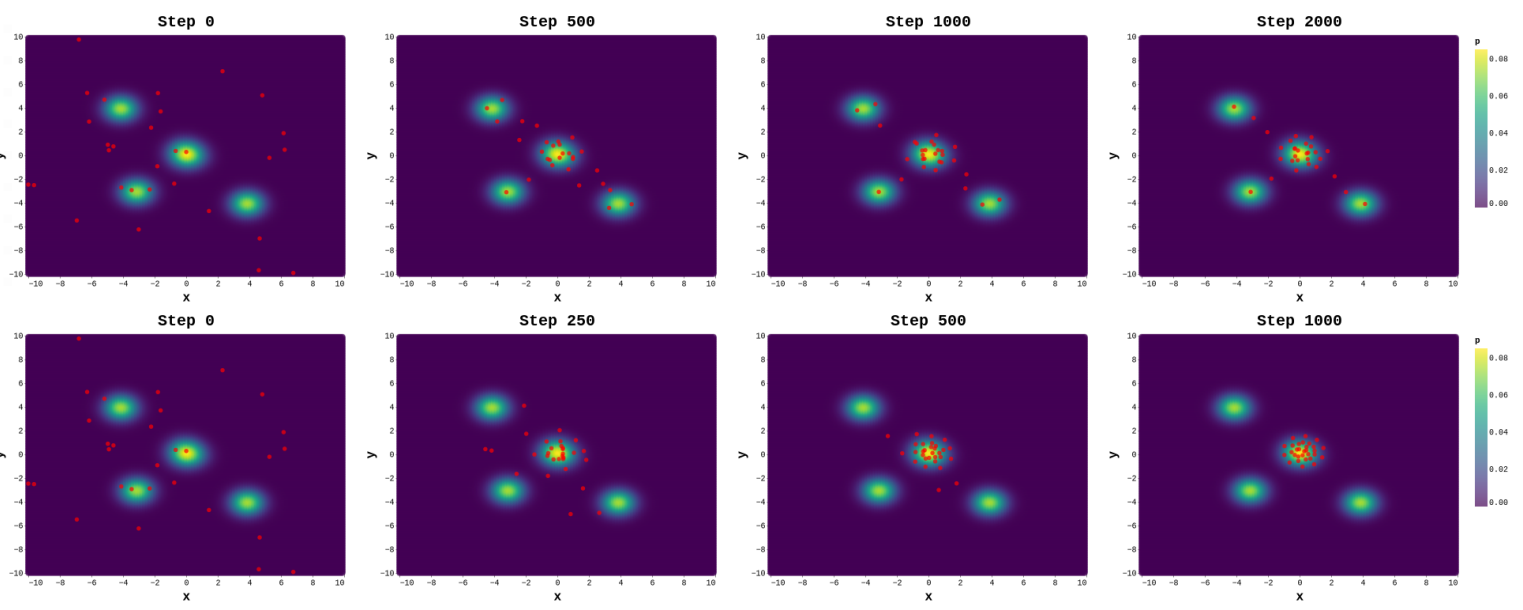
Figure 3: Sampling from three mixtures of two Gaussian distributions with a joint high-likelihood
region. We run MOO-SVGD (top) and MT-SGD (bottom) to update the initialized particles
(left-most figures) until convergence. While MOO-SVGD transports the
initialized particles scattering on the distributions, MT-SGD perfectly drives them to diversify in
the region of interest.

3.2 Multi-objective Optimization

The previous experiment illustrates that MT-SGD can be used to sample from multiple target distributions, we next test our method on the other low-dimensional multi-objectives OP. In particular, we use the two objectives ZDT3, whose Pareto front consists of non-contiguous convex parts, to show our method simultaneously minimizes both objective functions.

Figure 4: Solutions obtained by MOO-SVGD (mid) and MT-SGD (right) on ZDT3 problem after
10,000 steps, with blue points representing particles and red curves indicating the Pareto front. As
expected, from initialized particles (left), MOO-SVGD’s solution set widely distributes on the whole
Pareto front while the one of MT-SGD concentrates around middle curves (mostly the middle one).

3.3 Experiments on Multi-Fashion+Multi-MNIST Datasets
Our method is validated on different benchmark datasets: (i) Multi-Fashion+MNIST, (ii) Multi-MNIST, and (iii) Multi-Fashion. Each of them consists of 120,000 training and 20,000 testing images generated from MNIST and FashionMNIST by overlaying an image on top of another: one in the top-left corner and one in the bottom-right corner. Lenet (22,350 params) is employed as the backbone architecture and trained for 100 epochs with SGD in this experimental setup

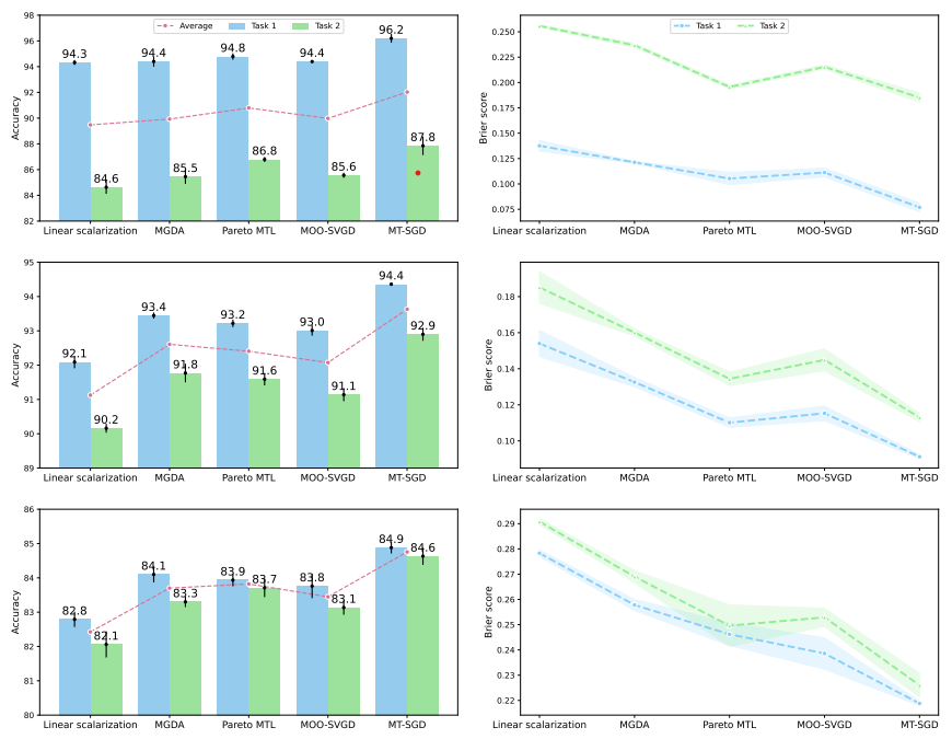
Figure 5: Results on Multi-Fashion+MNIST (left), Multi-MNIST (mid), and Multi-Fashion (right).
We report the ensemble accuracy (higher is better ) and the Brier score (lower is better ) over 3
independent runs, as well as the standard deviation (the error bars and shaded areas in the figures).

From the complexity point of view, MT-SGD introduces a marginal computational overhead compared to MGDA since it requires calculating the matrix $U$ , which has a complexity $O(K^2M^2d)$ , where the number of particles $M$ is usually set to a small positive integer. However, on the one hand, computing $U$ ‘s entries can be accelerated in practice by calculating them in parallel since there is no interaction between them during forward pass. On the other hand, the computation of the back-propagation is typically more costly than the forward pass. Thus, the main bottlenecks in our method lie on the backward pass and solving the quadratic programming problem – which is an iterative method

Figure 6: Running time on each epoch of MT-SGD and compared baselines on Multi-MNIST dataset.
Results are averaged over 5 runs, with the standard deviation reported by error bars.

3.4 Experiment on CelebA Dataset

We performed our experiments on the CelebA dataset, which contains images annotated with 40 binary attributes, we divide 40 target binary attributes into two subgroups: hard and easy tasks for easier visualization

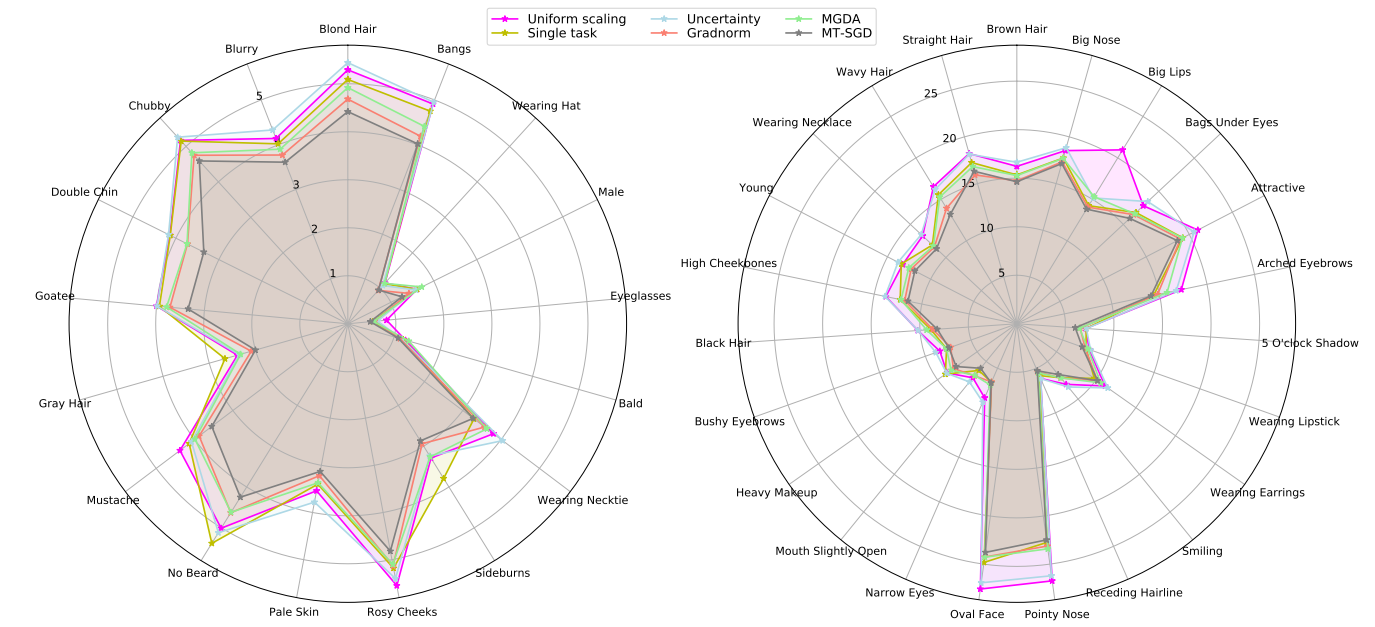
Figure 7: Radar charts of prediction error on CelebA for each individual binary classification
task. We divide attributes into two sets: easy tasks on the left, difficult tasks on the right

Compared to other baselines, our proposed method significantly reduces the prediction error in almost all the tasks, especially on “Goatee”, “Double Chi” and “No Beard”.

4. Conclusion

In this paper, we propose Stochastic Multiple Target Sampling Gradient Descent (MT-SGD), allowing us to sample the particles from the joint high-likelihood of multiple target distributions. Our MT-SGD is theoretically guaranteed to simultaneously reduce the divergences to the target distributions. Interestingly, the asymptotic analysis of our MT-SGD reduces exactly to the multi-objective optimization. We conduct comprehensive experiments to demonstrate that by driving the particles to the Pareto common (the joint high-likelihood of multiple target distributions), our MT-SGD can outperform the baselines on the ensemble accuracy and the well-known Bayesian metrics such as the expected calibration error and the Brier score.

References:

[1] Bishop, Christopher M. “Pattern recognition and machine learning (information science and statistics).” (2007): 183.
[2] Murphy, Kevin P. Probabilistic machine learning: an introduction. MIT press, 2022.
[3] Liu, Qiang, and Dilin Wang. “Stein variational gradient descent: A general purpose bayesian inference algorithm.” Advances in neural information processing systems 29 (2016).
[4] Welling, Max, and Yee W. Teh. “Bayesian learning via stochastic gradient Langevin dynamics.” Proceedings of the 28th international conference on machine learning (ICML-11). 2011.
[5] Désidéri, Jean-Antoine. “Multiple-gradient descent algorithm (MGDA) for multiobjective optimization.” Comptes Rendus Mathematique 350.5-6 (2012): 313-318.
[6] Mahapatra, Debabrata, and Vaibhav Rajan. “Multi-task learning with user preferences: Gradient descent with controlled ascent in pareto optimization.” International Conference on Machine Learning. PMLR, 2020.
[7] Sener, Ozan, and Vladlen Koltun. “Multi-task learning as multi-objective optimization.” Advances in neural information processing systems 31 (2018).
[8] Lin, Xi, et al. “Pareto multi-task learning.” Advances in neural information processing systems 32 (2019).
[9] Liu, Xingchao, Xin Tong, and Qiang Liu. “Profiling pareto front with multi-objective stein variational gradient descent.” Advances in Neural Information Processing Systems 34 (2021): 14721-14733.